[ Main page | About Your Results | About Genetic Algorithms | About Fuzzy Logic | The Importance of Explainability | Commercialising ]
This project was to construct a Minimum Viable Prototype (MVP) of an expert system for advising investors about start-up companies based on their Key Performance Indicators (KPIs). The system would be based on fuzzy-logic rules. The initial version of these would be written by a person, but the system would optimise it using machine learning: specifically, by using a genetic algorithm, "evolving" the rules to make them "fitter". In this context, that means making them better match the data that describes actual start-ups. I have demonstrated this in an extreme form, making the system learn by evolving rules from components that were complete rubbish. I consider this a success.
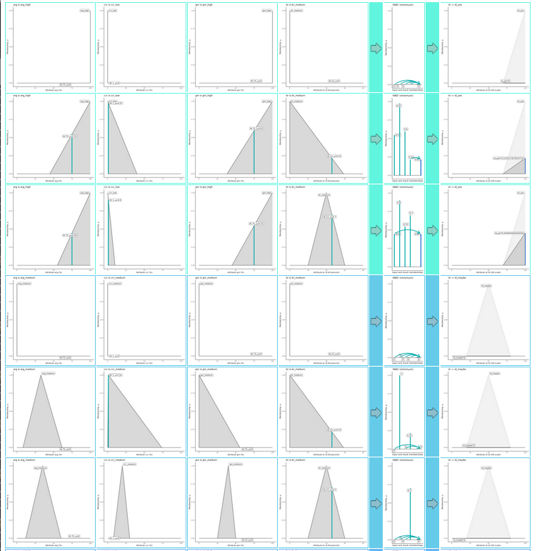
A short demonstration is given by the graphic
below. You will have seen something similar when
using the expert systems I pointed to for Stage 1
of the project. Each row diagnoses the application
of a rule. The graphs to the left of the first right-arrow
indicate how well the fuzzy sets in the rule
matched its inputs, and the final graph represents
how much weight this gives to the rule's conclusion.
In this particular image, rows are grouped
into threes as indicated by the colours. The
first row of a three shows how the starting
point for the evolution — the rubbish — did.
The second row shows how the result of evolving
from it did. And the third row shows how the
original knowledge base, which I hand-crafted,
did. Whether or not you know the details of
what the graphs mean, you can see that the
second row's are not too different from the third's,
while the first row's are very different from
both. In other words, the artificial evolution
has invented something not unlike the hand-crafted
version!

The rest of this page is divided into two sections. The first recaps on what I built for Stage 1 of the project. You have already seen the results, but I can now explain in rather more detail than before. The second section explains what I did for Stage 2, and how it follows on from Stage 1.
On the About Fuzzy Logic page, there's a section "Simple Investment-Attractiveness Expert System". This links to the input page for a conceptually simple system which relates one input attribute, Annual Revenue Growth, to one output attribute, Investment Attractiveness. The rules work the same way as the height-to-shoe-size rules earlier on the About Fuzzy Logic page, basically saying that the better is the revenue growth, the more attractive is the company.
One of the rules is `if arg be high then ia:=attractive`. This is obviously sensible. For my first experimental demonstration of computer evolution, I changed it to `if arg be low then ia:=attractive`. This is obviously not sensible. But my question was, could I demonstrate evolution changing it back to a better rule?
To do this, I first built a database to train it on. In real life, animals and plants are deemed fitter if they can escape from predators better, survive droughts longer, or whatever. In my artificial evolution, a rule is deemed fitter if it fits real data better. I didn't have any real data (you have to buy it), so I made some up. My made-up database contained data records with fields `arg` and `ia`, such that the records with higher `arg` also had, on average, higher `ia`. You can see these here. The database proper begins half-way down the first page, after some interface predicates.
I also wrote code to evolve the rule. I'll explain this in some detail, as it's relevant to Stage 2. You may find it helpful to read the explanation in conjunction with the About Genetic Algorithms page, particularly the article by Pico Finance.
Recall that the rule was `if arg be low then ia:=attractive`. The evolutionary code first generated an initial population of mutant rules from it. Each mutation tweaked the fuzzy set named `low`, making it perhaps a bit wider, or a bit shifted to the left, or a bit more skew, or whatever. The code then assessed the fitness of each mutant by running it over all the records in the database and finding how well the `ia` that it predicted from each record's `arg` matched the actual `ia`. Some mutants did slightly better than the original; others did worse.
The code then cycled through a succession of generations. The initial generation was the mutants just generated, plus the original rule. The code ordered them according to fitness, and then selected rules to breed from. Selection was probabilistic, so the fitter a rule, the more chance the code would give it to breed. Once the code had a breeding population, it combined rules pairwise — the first with the second, the third with the fourth, and so on.
When combining one rule with another, the code swaps parts of corresponding fuzzy sets. Imagine that rule A's `low` fuzzy set has its left vertex at 32, its apex at 35, and its right vertex at 37. Rule B's might have its at 31, 34, and 48. Then one way to cross them is to exchange apices so that one child becomes 32,34,37, while the other becomes 31,35,48.
This demonstrates two things. First, there are many ways to cross two rules — and indeed to mutate them. The designer of the algorithm, i.e. me, has to decide which from this multitude of possibilities to use, and with what probability. Second, crosses — and indeed mutations — can create invalid rules. If the second rule above had had apex 44, crossing it into the first rule would yield an invalid fuzzy set, its apex being to the right of its right vertex. The coder, i.e. me, has to test for an abundance of such cases, and it's an awful lot of work.
At any rate, after generating these pairs of children, the code probabilistically mutates each one. It then measures their fitness, and merges them with the population from which they were bred. The point here is that we want to take the fittest over to the next generation. While some offspring may be fitter than their parents and friends, some will be less fit. So everyone has to be assessed. Having done that, we can then take the fittest individuals — and that is the population with which we start the next generation.
Such an algorithm generates a huge number of individuals. To see how well its mutation and crossover operations are doing their job, we need to be able to "eyeball" the populations, and quickly compare one individual with another. So it's vital to have depictions which support this. For your runs, I was already outputting my diagnostics into web pages, because HTML makes formatting easy. In them, the individuals are rules, and the mutable entities within the rules are fuzzy sets. So I had to find a way to depict these for easy comparison amongst a very large population. Moreover, it seemed useful to be able to lay them vertically as well as horizontally, to save space. I decided to draw them, using Scalable Vector Graphics (SVG). This is a kind of pen plotter for the Web, where one moves a virtual pen to draw lines, polygons, circles, and other shapes. As you will see below, I output rules both as text and as SVG graphics.
With all the above in mind, I'll show off the output from a typical run. It's here. The headings point out the passage of generations, with their mutations and crossovers. Rules are shown as `if arg be trap(4.71,10.00,10.00,28.62) then ia:=trap(5.00,7.00,7.00,9.00)` , giving the numbers defining the fuzzy sets rather than their names. All set definitions are for trapezoids: the trapezoid `trap(A,B,C,D)` is a membership function which is 0 until A, then rises to 1 at B, stays 1 until C, drops to 0 at D, then stays 0. As it happens, I decided to simplify by making B and C identical, so that the trapezoids were triangles.
Populations are listed vertically, first as text and then as graphics. The text and graphics both run horizontally. To the left of each rule is its fitness: remember, this is how well it predicts the Investment Attractiveness values in the database, given Annual Revenue Growth. The numbers are such that lower fitness values indicate fitter rules.
You can see that the fitness numbers tend to decrease from generation to generation, meaning that the rules are getting fitter.
So this approach worked, and testing it on a single rule was a good simple way to begin. But after some more experiment, it started seeming as though it would be hard — within the time allowed for the project — to make fuzzy sets evolved this way work with multiple rules. Different rules would likely get evolved in different directions, and it could be hard to get a consistent set of fuzzy sets that worked for all of them.
So instead, I decided to treat the entire set of rules as a single entity, all members of which are governed by the same fuzzy sets. Instead of evolving the rules, I would evolve the fuzzy sets. Two rules mentioning the same fuzzy set might find evolution changes it, but both would see the same change. This helps maintain consistency between rules.
I first wrote a set of rules. I wanted these to use more attributes than just Annual Revenue Growth. That would make them more realistic, more interesting for you, and a better test of artificial evolution. On the other hand, if I had too many attributes, evolution would become too slow, and it would be harder to diagnose problems with the algorithm.
After some experiment, four attributes seemed about right. I chose:
I also chose two output attributes, relatives of the Investment Attractiveness used before. They were:
The rules I wrote to go with these are below:
if arg be arg_high and ccr be ccr_low and gm be gm_high and br be br_medium then id := id_yes.
if arg be arg_high and ccr be ccr_low and gm be gm_high and br be br_medium then rq := rq_medium.

if arg be arg_medium and ccr be ccr_medium and gm be gm_medium and br be br_medium then id := id_maybe.
if arg be arg_medium and ccr be ccr_medium and gm be gm_medium and br be br_medium then rq := rq_medium.

if arg be arg_high and ccr be ccr_low and gm be gm_high and br be br_low then id := id_yes.
if arg be arg_high and ccr be ccr_low and gm be gm_high and br be br_low then rq := rq_low.

if arg be arg_low and ccr be ccr_medium and gm be gm_medium and br be br_medium then id := id_no.
if arg be arg_low and ccr be ccr_medium and gm be gm_medium and br be br_medium then rq := rq_high.

if arg be arg_high and ccr be ccr_low and gm be gm_high and br be br_low then id := id_yes.
if arg be arg_high and ccr be ccr_low and gm be gm_high and br be br_low then rq := rq_low.
To make these rules complete, we need to assign each fuzzy set — `arg_high`, `ccr_low`, etc. — a membership function. The values I chose are shown in this table:
| arg | br | ccr | gm | id | rq | |
|---|---|---|---|---|---|---|
| low | 0.00 | 0.00 | 0.00 | 0.00 | 0.00 | 0.00 |
| high | 100.00 | 40.00 | 100.00 | 100.00 | 100.00 | 10.00 |
| down | 15.00 | 15.00 | 10.00 | 30.00 | 30.00 | 3.00 |
| up | 55.00 | 25.00 | 28.00 | 45.00 | 70.00 | 7.00 |
| triA | 12.00 | 10.00 | 8.00 | 25.00 | 20.00 | 2.00 |
| triB | 35.00 | 20.00 | 20.00 | 40.00 | 50.00 | 5.00 |
| triC | 60.00 | 30.00 | 30.00 | 50.00 | 80.00 | 8.00 |
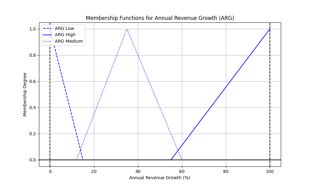
Here, `low` and `high` are the domain boundaries. All scales are
percent, and all attributes except Burn Rate end at 100%. Burn Rate
terminates earlier, because burn rates higher than 40% may indicate
a very serious problem, which I've not made the rules handle.
The `tri` rows define the three vertices of a triangular membership
function, `triA` being left and `triB` being the apex. Finally,
`down` defines a set descending from a membership of 1 at the
domain low boundary to the value given; `up` is the converse, a
set that rises from 0 at the value given up to 1 at the domain
high boundary. If this is not clear, please look at membership
functions again in the links from
About Fuzzy Logic, and at the
graph below. Look at where the sloping lines' X-values are when
their membership degree is 0 or 1, and compare with the `arg` column in the
above table.

I now had to make another database. This time, it would have four input attributes and two output ones, rather than one input and one output. This is fairly easy to visualise, if we think of each start-up as a point in a four-dimensional hypercube whose axes are labelled ARG, CCR, GM, and BR. We can tag each point with its ID and RQ values, perhaps by giving each one a colour (red for yes, blue for no) and a taste (sweet for not risky, sour for risky).
Looking at the hypercube, we'll see there are various clusters, each with its own shape. Some of those shapes may express correlations between attributes. For example, if ARG and GM are correlated, we might expect to be able to fit a region stretching from coordinates where ARG and GM are both high to those where they are both low. Crawling around in the hypercube while simultaneously looking at and licking the start-ups, you get a pretty good feel for their distribution.
How could I build a database containing such clusters? For this simple experiment, I synthesised it from my rules. I wrote code to take a rule and loop over the fuzzy sets it mentioned. For each fuzzy set, it chose a point at random. The selection was biased, so that for the triangular fuzzy sets, the greatest probability was at the apex, dropping off along each slope to zero probability at the left and right vertices. (This is, in fact, a triangular probability distribution.) Selecting points for the `up` and `down` sets was like selecting for half a triangle: highest probability where membership was 1, dropping off to zero where it was 0. The result can be seen here. It should also be mentioned that I sized each cluster according to the proportion of companies of that type expected.
Of course, in real life, we'd buy a database. But for this experiment, I just needed data that, when used as training data, I could be reasonably sure would allow me to recreate my original rules if my training method was any good.
The most impressive results are in run 5 and run 6. Here, I wanted to see whether the genetic algorithm could discover the fuzzy sets from scratch. That is, if I started it off with sets that bore no relation at all to the data, could it learn solely from the database what those sets should be, without any hints from existing definitions?
These are the sets I started with. As you can see, I have given all their X points dummy values: either an extreme low or an extreme high. Basically, this makes all the sets into spike functions:
| arg | br | ccr | gm | |
|---|---|---|---|---|
| low | 0.00 | 0.00 | 0.00 | 0.00 |
| high | 100.00 | 40.00 | 100.00 | 100.00 |
| down | 0.00 | 0.00 | 0.00 | 0.00 |
| up | 99.99 | 39.99 | 99.99 | 99.99 |
| triA | 0.00 | 0.00 | 0.00 | 0.00 |
| triB | 0.00 | 0.00 | 0.00 | 0.00 |
| triC | 0.00 | 0.00 | 0.00 | 0.00 |
I then ran the fuzzy-set evolver on them. Run 6 used a population size of 100 over 200 generations. Or would have done. It actually crashed Prolog in generation 110, probably because of memory problems. The run is here, and I reshow the fittest individual therein at this stage below. Searching the file for "Evolving Generation 110" will find it, displayed just after some headings:
| arg | br | ccr | gm | |
|---|---|---|---|---|
| low | 0.00 | 0.00 | 0.00 | 0.00 |
| high | 100.00 | 40.00 | 100.00 | 100.00 |
| down | 18.92 | 14.71 | 39.90 | 0.66 |
| up | 44.80 | 29.14 | 74.32 | 38.24 |
| triA | 8.21 | 0.00 | 0.00 | 0.00 |
| triB | 32.60 | 0.00 | 0.95 | 0.00 |
| triC | 61.42 | 29.30 | 73.64 | 55.51 |
There is another such run here. This one ran for less time with fewer individuals, but still managed a reasonable amount of evolution. To try the sets discovered above for yourself, please go to https://expertsystemdemos.net/chaves_triplex.php. This is the "triplex" version of the expert system, the one that generated the graphics shown at the head of this report, and that compares the nonsensical fuzzy sets, the sets evolved from them, and the hand-crafted originals.